Intro to Postgre EXPLAIN
Table of Contents
For most of the database performance work I have done, simply looking at the queries has been enough to identify the issue. However, I’ve been tempted by the additional information that the EXPLAIN function can provide. Unfortunately, I didn’t understand the output of these queries and would inevitably go back to other avenues when debugging issues. I decided to change that and learn how to work with EXPLAIN.
Please note, while other database management systems provide EXPLAIN functionality, it is not SQL standard. I will be focusing on how it works with PostgreSQL since that is what I use most often; you will want to read the documentation for your DBMS of choice if you work with a different system.
What is EXPLAIN
To start, EXPLAIN is a SQL function that, when given a query, will return the database’s plan of how to fetch the data. It does not actually perform the query you pass into it.
EXPLAIN(
  SELECT *
  FROM my_table
);

                            QUERY PLAN
------------------------------------------------------------------
 Seq Scan on my_table  (cost=0.00..10.50 rows=50 width=1572)
(1 row)
You can think of the query plan as map directions. It includes the steps you will be taking to get your requested data from the database.
However, you will not be getting information about the distance before you turn left or how long you will be on a highway. Instead, you will get information about the steps involved in fetching your data and how much work will be done along the way.
Our simple example above only has one step in our directions list – a sequential scan on my_table. Even for this single step, we get a lot of data about what will be happening.
Seq Scan on my_table (cost=0.00..10.50 rows=50 width=1572)
Let’s break down what is involved in a row from the query planner.
Reading from the Table
Our query plan indicates which table we will be reading data from and the method used to read said data.
Seq Scan on my_table
In this example, we will be doing a sequential scan on my_table. A sequential scan requires reading each row in the table, one by one. Check out this post for more information on the different types of table scans.
Statistics Tuple
After the scan information, we have a tuple (()) of statistics. This includes cost, rows, and width.
(cost=0.00..10.50 rows=50 width=1572)
Cost
First in our tuple is cost.
cost=0.00..10.50
The cost contains two numbers; 0.00 and 10.50 in this case.
Start-up
The first number is the estimated start-up cost; this is the cumulative cost before this step in the plan will run. In our example, the start-up cost is 0.00. A start-up cost of 0.00 indicates that the step runs at the beginning of the query execution. Since we only have a single step in our example, it makes sense intuitively that it will run at the beginning of execution.
Let’s take a look at a slightly more complex query. In this example, our WHERE clause is filtering based on a subquery.
EXPLAIN(
  SELECT *
  FROM chat_room_messages
  WHERE author IN (
    SELECT email
    FROM users
    WHERE updated_at > '2021-01-01'::date
  )
);
This results in a plan with multiple steps.
QUERY PLAN
-----------------------------------------------------------------------------
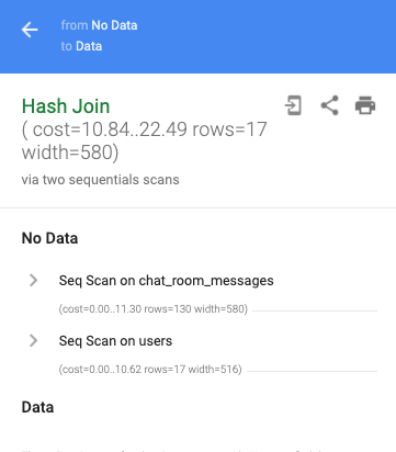
Hash Join (cost=10.84..22.49 rows=17 width=580)
Hash Cond: ((chat_room_messages.author)::text = (users.email)::text)
-> Seq Scan on chat_room_messages (cost=0.00..11.30 rows=130 width=580)
-> Hash (cost=10.62..10.62 rows=17 width=516)
-> Seq Scan on users (cost=0.00..10.62 rows=17 width=516)
Filter: (updated_at > '2021-01-01'::date)
As we said before, when the estimated start-up cost is 0.00, it is an indication that that step is run at the beginning of execution. The plan above has two rows with 0.00 for the estimated start-up cost.
                                 QUERY PLAN
-----------------------------------------------------------------------------
 Hash Join  (cost=10.84..22.49 rows=17 width=580)
   Hash Cond: ((chat_room_messages.author)::text = (users.email)::text)
   ->  Seq Scan on chat_room_messages  (cost=0.00..11.30 rows=130 width=580)
   ->  Hash  (cost=10.62..10.62 rows=17 width=516)
         ->  Seq Scan on users  (cost=0.00..10.62 rows=17 width=516)
               Filter: (updated_at > '2021-01-01'::date)
We have the sequential scan on the chat_room_messages table
-> Seq Scan on chat_room_messages (cost=0.00..11.30 rows=130 width=580)
and we also have a sequential scan on the users table
-> Seq Scan on users (cost=0.00..10.62 rows=17 width=516)
This is an indication we will start these two steps at the same time and run them in parallel.
Total
The second number in cost is the estimated total cost, the accumulated cost after the step completes.
Together, the numbers in cost give us an idea of when the step will start and when it will end.
Nesting
Let’s use what we know about cost to revisit our complex query plan.
->  Hash  (cost=10.62..10.62 rows=17 width=516)
  ->  Seq Scan on users  (cost=0.00..10.62 rows=17 width=516)
    Filter: (updated_at > '2021-01-01'::date)
Not only does this example have multiple steps, but it also has nested steps.
To understand what runs first, we will rely on our knowledge that an estimated start-up cost of 0.00 means a step is run when execution starts. For the query above, Seq Scan on users has an estimated start-up cost of 0.00; this means it runs first. It also has an estimated total cost of 10.62.
Moving onto the Hash line above, we see that its estimated start-up cost is 10.62. This means that as soon as the seq scan on users completes, it will move on to the Hash step.
->  Hash  (cost=10.62..10.62 rows=17 width=516)
  ->  Seq Scan on users  (cost=0.00..10.62 rows=17 width=516)
Through our understanding of the cost attribute, we have been able to piece together an understanding for one of the fundamental aspects of a query plan’s layout - that it represents a tree-like structure where the leaf nodes (the most nested elements) are run first.
You may be wondering about the Filter line. Note that it isn’t prefixed with an ->; this means that it isn’t a separate step in our plan. Instead, it is a part of our scan on the users table. This means that Seq Scan on users is still our most nested step.
How Much?
So far, we have covered what the two types of cost represent but not what the values represent. While we’ve talked about the cost as a sort of time-like measurement, it is not a representation of time. The unit used for cost is configurable but defaults to representing sequential page fetches. However, the units are arbitrary; what matters is the relative costs. From the postgreSQL documentation
The cost variables described in this section are measured on an arbitrary scale. Only their relative values matter, hence scaling them all up or down by the same factor will result in no change in the planner’s choices
So while you may want to track the cost in terms of sequential page fetches or base it on the CPU processing a tuple, what seems to be more important is comparing the numbers relative to other parts of the query plan (and other query plans).
Rows
The next part of our tuple is rows.
rows=50
rows represents the estimated number of rows that will be returned for a given step. Since EXPLAIN will not run the query, it cannot specify exact numbers. Instead, it uses statistics gathered from the ANALYZE function and stored in a special table. Despite being an estimation, it can provide a ballpark of how much data you may be dealing with and how impactful a filter may be.
Width
The final element of the query plan tuple that we are going to cover is width.
Seq Scan on my_table (cost=0.00..10.50 rows=50 width=1572)
The width is the average width of the rows in bytes. More than just the number of columns selected, it gives you an idea of the average amount of data stored in those columns. Like rows, it is an estimation based on the statistics table.
While you would expect that selecting fewer columns results in less data, EXPLAIN can help reveal which columns have the largest memory footprint. When we perform a SELECT * we see a much larger width than if we only SELECT id.
-- SELECT * has a width of 580
# EXPLAIN(SELECT * FROM chat_room_messages);

                              QUERY PLAN
-----------------------------------------------------------------------
 Seq Scan on chat_room_messages  (cost=0.00..11.30 rows=130 width=580)
(1 row)

-- SELECT id has a width of 8
# EXPLAIN(SELECT id FROM chat_room_messages);

                             QUERY PLAN
---------------------------------------------------------------------
 Seq Scan on chat_room_messages  (cost=0.00..11.30 rows=130 width=8)
(1 row)
Analyze
As previously mentioned, EXPLAIN will not run the query you pass in. This is why we’ve been dealing with estimations so far. If you want to get more accurate performance information, you can use EXPLAIN ANALYZE. With ANALYZE, the query will actually be run, allowing the query plan to include information about run time, the actual number rows, and more.
Let’s take a look at one of our previous queries and include an ANALYZE.
EXPLAIN ANALYZE(
  SELECT *
  FROM chat_room_messages
  WHERE author IN (
      SELECT email FROM users WHERE updated_at > '2021-01-01'::date
  )
);

                                                       QUERY PLAN
------------------------------------------------------------------------------------------------------------------------
 Hash Join  (cost=10.84..22.49 rows=17 width=580) (actual time=0.028..0.033 rows=10 loops=1)
   Hash Cond: ((chat_room_messages.author)::text = (users.email)::text)
   ->  Seq Scan on chat_room_messages  (cost=0.00..11.30 rows=130 width=580) (actual time=0.007..0.008 rows=10 loops=1)
   ->  Hash  (cost=10.62..10.62 rows=17 width=516) (actual time=0.009..0.009 rows=2 loops=1)
     Buckets: 1024  Batches: 1  Memory Usage: 9kB
     ->  Seq Scan on users  (cost=0.00..10.62 rows=17 width=516) (actual time=0.005..0.005 rows=2 loops=1)
       Filter: (updated_at > '2021-01-01'::date)
 Planning Time: 0.104 ms
 Execution Time: 0.050 ms
(9 rows)
While the overall plan is the same as before, we now have additional information next to our cost, rows, width tuple. This new tuple gives us our actual runtime statistics.
In addition to our arbitrary units for cost, we now get time (in milliseconds). We also get to see the actual number of rows returned. We can see some steps where the planner was close (17 versus 10) and others less so (130 versus 10). These examples come from a small test database that is not getting regular ANALYZE runs; as a result, the previously mentioned statistics table used for estimations will be less helpful.
We also have new information about our hash function (number buckets, amount of memory used) and the overall run time (planning versus actual execution).
ANALYZE provides valuable information on top of only using EXPLAIN. However, because it does require running the query, it will take longer. This extended runtime may make it difficult to use repeatedly for large queries.
Caveats
Matching Environments
The biggest caveat I took away from the documentation is that query plans are specific to the amount of data in the database. As a result, running an EXPLAIN locally with a small dataset may not reveal the steps the query planner will take on your production system.
An example of how the planner will choose different routes is index utilization. With a small enough table, the query planner may prefer a sequential scan over leveraging an index. As a result, you may not be able to confirm the usage of a newly added index in your smaller development database.
From what I can tell, the query plan is impacted primarily by the amount of data and not other factors like the underlying hardware. As a result, you should be able to get a better idea of production-like characteristics if you load your local database with enough data (if feasible). However, like many performance tuning tasks, you will ultimately want to validate on production.
Reading and Writing
Another thing to note is that plans focus on reading and do not include information about updates. In the example below, we run EXPLAIN on an UPDATE command.
EXPLAIN
UPDATE chat_room_messages
SET body = 'this is an updated message'
WHERE id = 1;

                                                QUERY PLAN
----------------------------------------------------------------------------------------------------------
 Update on chat_room_messages  (cost=0.14..8.16 rows=1 width=586)
   ->  Index Scan using chat_room_messages_pkey on chat_room_messages  (cost=0.14..8.16 rows=1 width=586)
         Index Cond: (id = 1)
(3 rows)
The query plan includes information about scanning the table but does not include any cost information for performing the update itself.
With EXPLAIN ANALYZE, the actual time shows a gap between the scan and the overall runtime, so you may be able to estimate how long the `UPDATE is taking.
                                                                     QUERY PLAN
----------------------------------------------------------------------------------------------------------------------------------------------------
 Update on chat_room_messages  (cost=0.14..8.16 rows=1 width=586) (actual time=0.055..0.055 rows=0 loops=1)
   ->  Index Scan using chat_room_messages_pkey on chat_room_messages  (cost=0.14..8.16 rows=1 width=586) (actual time=0.021..0.022 rows=1 loops=1)
         Index Cond: (id = 1)
 Planning Time: 0.064 ms
 Execution Time: 0.076 ms
(5 rows)
Conclusion
Hopefully, this introduction will empower you to leverage the EXPLAIN function. If you find a confusing query plan or struggle to know how to leverage the query plan to do something actionable, remember this quote from the documentation:
Plan-reading is an art that requires some experience to master